Anti-reflection coating design (gradient-based inverse design)

What this is

A three-layer dielectric anti-reflection (AR) coating on a high-permittivity substrate (εr = 12), designed automatically by gradient descent through the FDTD solver. The design variables are the three layer permittivities; the objective is the X-band-mean reflection off the coated substrate. A standard gradient-descent optimizer (Adam) drives that objective down through the differentiable forward model, and the converged cost is checked against the exact transfer-matrix optimum for the same layer count.

Unlike the other gallery cases, the headline here is not a single S-parameter curve checked against theory — it is the optimization loop itself: the cost falls from its starting value to within a few percent of the closed-form multilayer optimum, using only jax.grad of the FDTD reflection. That gradient is what makes the design loop possible.

What you’ll learn

• Posing an inverse-design problem: pick design variables (three layer εr), a scalar objective (band-mean reflection), and let the gradient drive the layers.
• Running gradient descent on jax.value_and_grad of an FDTD-computed reflection cost — the same solver gradient the other cases check once, here closed into a 60-iteration design loop.
• Reading a convergence curve and a per-layer εr trajectory, and understanding why the validated quantity is the scalar cost, not the individual layer values.
• Cross-checking the converged cost against the exact transfer-matrix optimum — and why a band-mean reflection target admits many equally good coatings (distinct layer combinations reaching the same cost).

Geometry & materials

A high-permittivity substrate (εr = 12, the kind of dielectric loading used under printed structures) reflects strongly at an air interface. Three quarter- wave-scale dielectric layers are stacked between air and the substrate; their permittivities are the knobs the optimizer turns.

import numpy as np
C0 = 299_792_458.0

eps_substrate = 12.0        # high-index substrate to be matched
n_layers      = 3           # three dielectric matching layers
band          = (8.0e9, 12.0e9)   # X-band reflection target
dx            = 0.5e-3      # 0.5 mm cells
# design variables: the three layer permittivities eps1, eps2, eps3

The layer thicknesses are held fixed; only the three permittivities are optimized. Each layer’s εr enters the FDTD permittivity grid as a continuous value, so the reflection cost is a smooth, differentiable function of the design vector.

Source, ports, boundaries, mesh

• Broadband plane-wave (TFSF) source. A total-field/scattered-field boundary injects a clean forward plane wave spanning X-band; the reflected field is read in the scattered-field region ahead of the stack.
• CPML on the propagation axis. A thick absorber terminates both ends so the reflection read is the coating’s, not an absorber artefact.
• Reflection cost = X-band-mean reflected power. A single temporal DFT over the reflected field gives the reflection spectrum; the scalar objective is its mean over the X-band target.
• 0.5 mm uniform mesh, 3147 time steps per forward solve. Each optimizer iteration is one differentiable forward solve (cost and gradient together); 60 iterations make up the run.

Note

The objective is a band-mean reflection, so several distinct layer-permittivity triples reach essentially the same cost. The loop converges in cost, not to one specific coating — see Validation & limits.

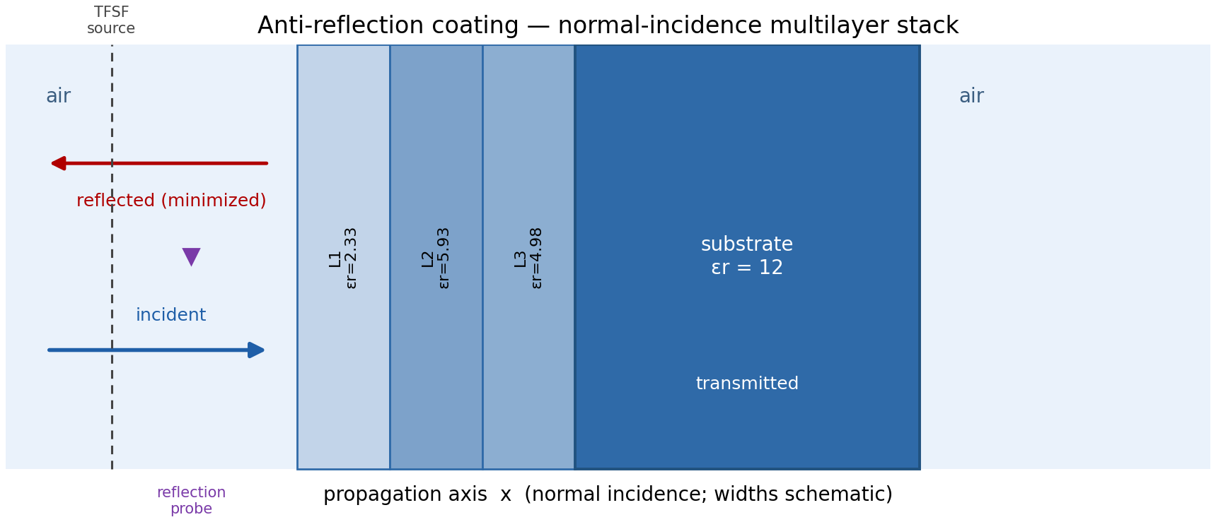
Geometry check (before running)

The render above confirms the stack before committing compute: air on the left, the three matching layers, and the εr = 12 substrate, with the TFSF plane and the reflection probe in clear space ahead of the coating and clearance to the CPML on both ends.

Run

Each design step evaluates the FDTD reflection cost and its gradient with respect to the three layer permittivities; the optimizer updates the design and the loop repeats.

python scripts/precompute_gallery_artifacts.py --case ar_coating_design

The optimization trace (per-iteration cost and the three layer permittivities) is emitted as machine-readable JSON alongside the figures.

Optimization trace (JSON) Per-iteration cost and the three layer permittivities over the 60-iteration optimization run.

Fields

This is a one-dimensional normal-incidence problem — the FDTD domain is a single cell thick transversely — so there is no 2-D field map; the field is the standing wave along the propagation axis. With the matching layers in place the reflected branch ahead of the stack is small (the optimizer minimizes it) and most of the incident power passes into the εr = 12 substrate. The field is best seen co-evolving with the design — the animation in the optimization section below shows the reflected field ahead of the stack shrinking as the optimizer tunes the three layers.

Result

The converged spectrum: the X-band reflection of the optimized 3-layer coating, against the bare εr = 12 substrate and the exact transfer-matrix optimum for the same layer count. The optimized stack suppresses the bare-substrate reflection across the band, sitting close to the closed-form multilayer optimum.

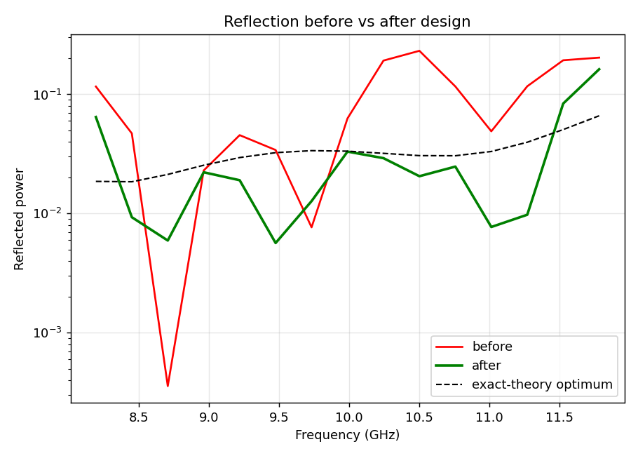
The single number that is validated is the band-mean reflection cost: the converged FDTD design reaches a final cost of 3.40e-02, which is 0.99x the exact transfer-matrix optimum (3.43e-02) — the gradient-driven design lands essentially on the closed-form optimum for this layer count.

Validation & limits

The validated quantity is a scalar: the X-band-mean reflection cost ratio of the converged FDTD design to the exact transfer-matrix optimum. The reference is the analytic transfer-matrix (exact-theory) optimum for a 3-layer stack.

Observable	rfx	Reference	Agreement	Pass
Band-mean reflection cost	3.40e-02	3.43e-02 (analytic transfer-matrix optimum)	ratio <= 1.2x	yes
Cost ratio to transfer-matrix optimum	0.99x	1.00x (exact theory)	<= 1.2x	yes
Cost ratio to quarter-wave ladder	0.50x	—	<= 0.7x	yes

Reference: the analytic transfer-matrix optimum. What is checked here is optimization convergence, not a single-frequency error bound: the converged cost must land within 1.2x of the transfer-matrix optimum, and it must clearly beat the plain quarter-wave-ladder starting design (below 0.7x of its cost). Both hold with room to spare — 0.99x the optimum and 0.50x the ladder.

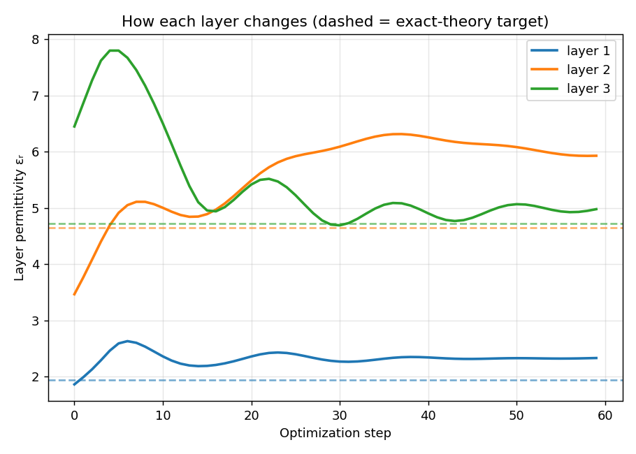
Many coatings, one cost. Because the objective is a band-mean reflection, multiple distinct layer-permittivity triples reach essentially the same cost. The converged FDTD design (εr ≈ [2.33, 5.93, 5.01]) and the transfer-matrix optimum (εr ≈ [1.94, 4.65, 4.72]) differ layer-by-layer while landing at nearly the same cost. So the cost is validated against exact theory; the individual layer values are one member of an equal-cost family, not a single “true” coating. The claim is convergence-in-cost, not design recovery.

Limits. The cost is the FDTD band-mean reflection at the run mesh (0.5 mm); the layer thicknesses are fixed and only the three permittivities are optimized. A finer mesh or a larger design space (thicknesses, more layers) would shift the absolute cost, but the convergence-to-theory picture is what this case demonstrates.

Autodiff — the optimization loop

This is where the differentiable FDTD does the work. The design loop is plain gradient descent: at each iteration a single jax.value_and_grad call returns both the band-mean reflection cost and its gradient with respect to the three layer permittivities — differentiated automatically back through every Yee update of the forward solve — and the optimizer steps the design down that gradient. No adjoint solver is hand-written; the gradient comes out of the solver itself.

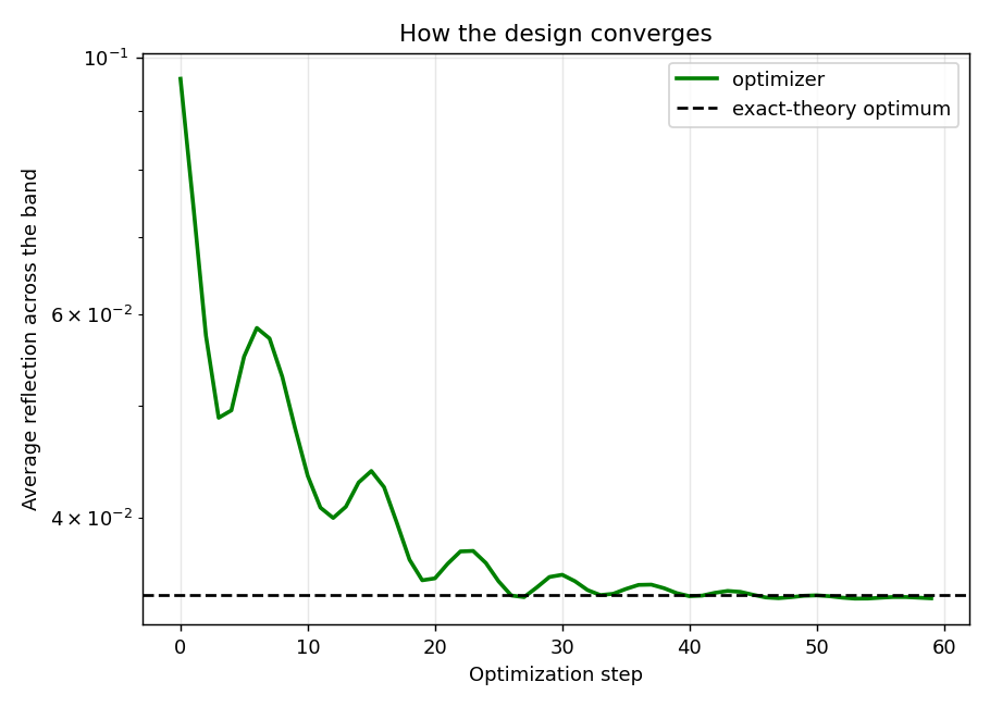
The convergence curve shows the band-mean reflection cost falling over the 60 iterations, from a starting cost near 9.6e-02 to the converged 3.40e-02, settling onto the exact transfer-matrix optimum line:

The per-layer trajectory shows the three permittivities moving together as the gradient reshapes the stack. They settle into a basin rather than onto a single sharp point — the visible signature of the many-designs-one-cost objective: the cost is pinned long before the individual layers stop drifting.

The two views together — the design and the field it produces — co-evolving as the optimizer iterates: the three-layer εr profile reshapes while the reflected field ahead of the stack shrinks, iteration by iteration.

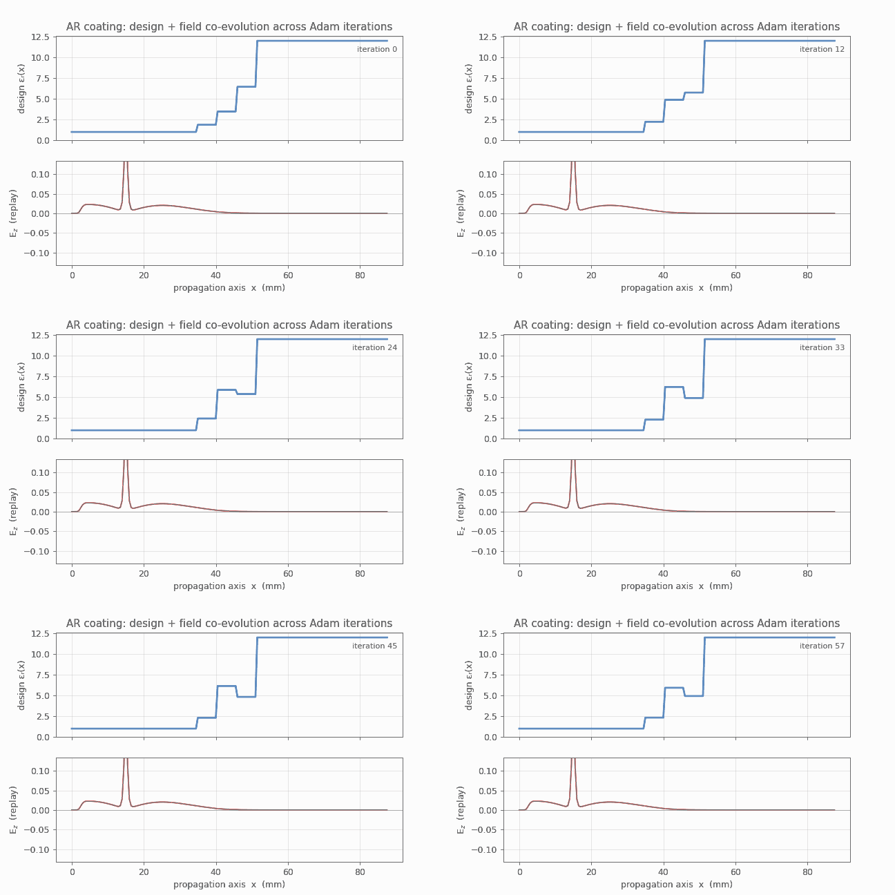
The gradient that drives all of this is the same solver gradient the other gallery cases check against finite differences for a single derivative; here it is closed into a loop. Because the cost is differentiable in the three layer permittivities, the optimizer never needs a finite-difference sweep of the design space — the descent direction comes directly from jax.grad of the FDTD cost.

Next

Dielectric slab (normal incidence) Reflection and transmission of a dielectric slab vs the exact transfer-matrix solution, with the AD gradient dT/dd cross-checked against the closed-form derivative.

Rectangular microstrip patch antenna (2.4 GHz, FR4) A printed resonator: matched return-loss dip, resonance vs the analytic transmission-line estimate, and a differentiable substrate sweep.

Computed with rfx · 2026-06-30