Dielectric slab (normal incidence)

What this is

A single lossless dielectric slab (εr = 4, refractive index n = 2) of finite thickness d sitting in free space, with a plane wave at normal incidence. Part of the wave reflects off the front face and part transmits through. The reflected and transmitted power follow the exact slab transfer matrix; the slab is transparent (R = 0, T = 1) whenever it is an integer number of half-wavelengths thick — the Fabry–Pérot condition n·d = m·λ₀/2 for m = 1, 2, 3, ….

What you’ll learn

• Driving a plane wave into a layered medium with a total-field/scattered-field (TFSF) source.
• Reading reflection R = |S11|² and transmission T = |S21|² from the scattered and total fields.
• Recognising the Fabry–Pérot transmission peak where the slab is a half-wave thick.
• Cross-checking rfx against the exact transfer-matrix solution and confirming energy conservation R + T = 1 on a lossless slab.

Geometry & materials

The slab is the only structure; everything else is vacuum. The 1D physics is captured in a thin 2D TMz strip with periodic top/bottom boundaries, so the wave sees an infinite slab at normal incidence.

import numpy as np
C0 = 299_792_458.0

eps_slab = 4.0          # slab relative permittivity (n = 2)
d_slab   = 10.0e-3      # slab thickness: 10 mm
dx       = 1.0e-3       # 1 mm cells -> 10 cells across the slab

# half-wave (Fabry-Perot) frequency: n*d = lambda0/2
n_slab   = np.sqrt(eps_slab)
f_fp     = C0 / (2 * n_slab * d_slab)        # ~7.5 GHz, slab transparent
# -> n = 2.0, first transmission peak near 7.5 GHz

A 10 mm slab of n = 2 is a half-wavelength thick near 7.5 GHz, so that is where the reflection vanishes and the slab passes the wave cleanly.

Source, ports, boundaries, mesh

• TFSF plane-wave source. A total-field/scattered-field boundary injects a clean forward plane wave. The reflected wave is read in the scattered-field region ahead of the slab; the transmitted wave is read in the total-field region behind it.
• CPML on the propagation axis (20 cells). The wave must leave the domain on both ends without re-entering; a thick absorber keeps the back-reflection well below the ~1% measurement floor across the whole band.
• Periodic transverse boundaries. A normal-incidence plane wave has no transverse variation, so one cell across the width with periodic walls reproduces the infinite-slab problem at a fraction of the cost.
• 10 cells across the slab. At 1 mm cells the 10 mm slab is resolved with ten cells, and the half-wave field variation inside it is well sampled up to the top of the band.

Note

Because the geometry is one-dimensional, this whole case runs in seconds on a CPU — no GPU required.

Geometry check (before running)

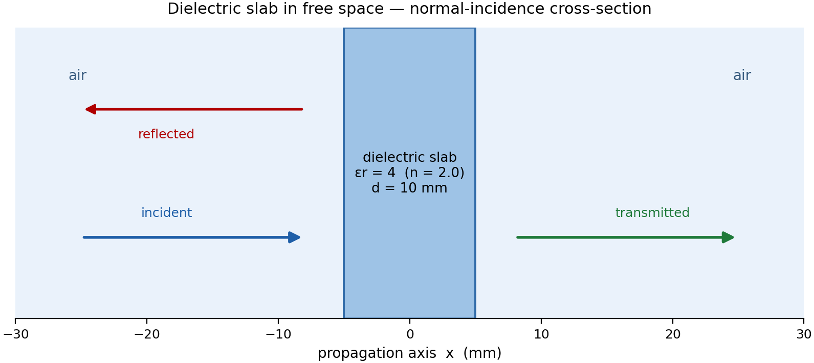
The cross-section above confirms the setup before committing compute: a single 10 mm slab centred in free space, with the incident wave from the left, the reflection heading back, and the transmission continuing through. The probes sit in clear air on either side, away from the absorber.

A 600-cell strip run over a few hundred steps finishes in a couple of seconds on a CPU; peak memory is a few megabytes.

Run

A broadband Gaussian plane wave covers roughly 3–12 GHz in one shot. The scattered field ahead of the slab gives R; the total field behind it gives T.

from rfx.grid import Grid
from rfx.core.yee import init_state, init_materials, update_e, update_h
from rfx.boundaries.cpml import init_cpml, apply_cpml_e, apply_cpml_h
from rfx.sources.tfsf import (
    init_tfsf, update_tfsf_1d_h, update_tfsf_1d_e, apply_tfsf_e, apply_tfsf_h,
)

grid = Grid(freq_max=20e9, domain=(600 * dx, 0.004, dx), dx=dx,
            cpml_layers=20, mode="2d_tmz")
dt = grid.dt

# broadband plane wave, +x, Ez-polarised
tfsf_cfg, tfsf_st = init_tfsf(grid.nx, dx, dt, cpml_layers=20, tfsf_margin=5,
                              f0=10e9, bandwidth=0.5, polarization="ez",
                              direction="+x", ny=grid.ny, nz=grid.nz)

# stamp the slab into the permittivity
slab_lo = grid.nx // 2 - int(d_slab / (2 * dx))
slab_hi = grid.nx // 2 + int(d_slab / (2 * dx))
materials = init_materials(grid.shape)
materials = materials._replace(
    eps_r=materials.eps_r.at[slab_lo:slab_hi, :, :].set(eps_slab))

state = init_state(grid.shape)
cp, cs = init_cpml(grid)
# ... step the Yee update, record E_z at a reflection probe and a
#     transmission probe, then FFT to get R(f) and T(f) ...

Run it from the command line:

python scripts/precompute_gallery_artifacts.py --case multilayer_fresnel

Fields

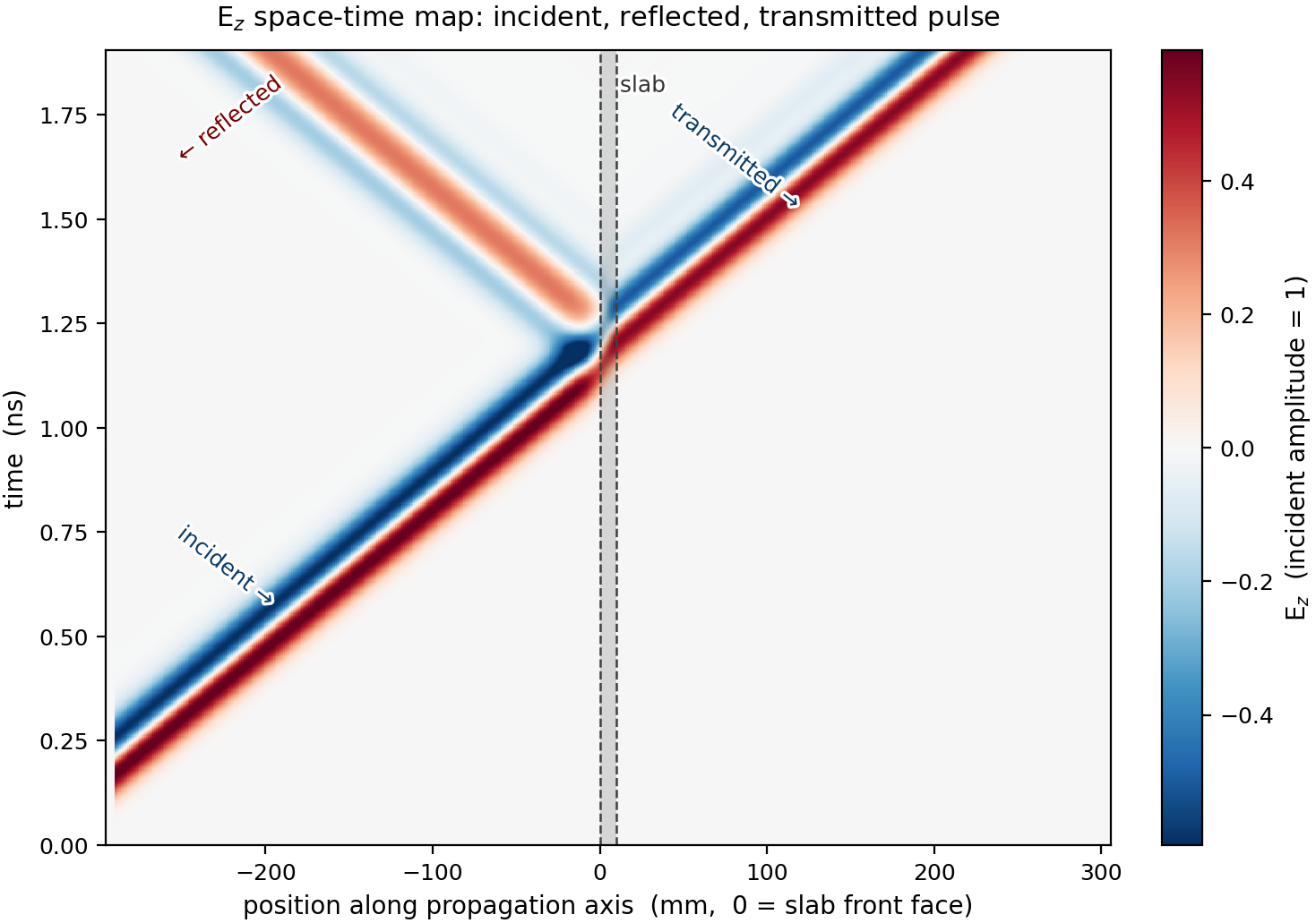
The space-time map below shows E_z along the propagation axis (horizontal) as time advances (vertical). The incident pulse travels at c through the air and hits the front face of the slab. There it splits: part reflects (the branch that turns back toward the source) and part transmits (the branch that continues forward, with a kink in slope inside the slab where the wave slows to c/n). The two outgoing branches are the R and T measured below.

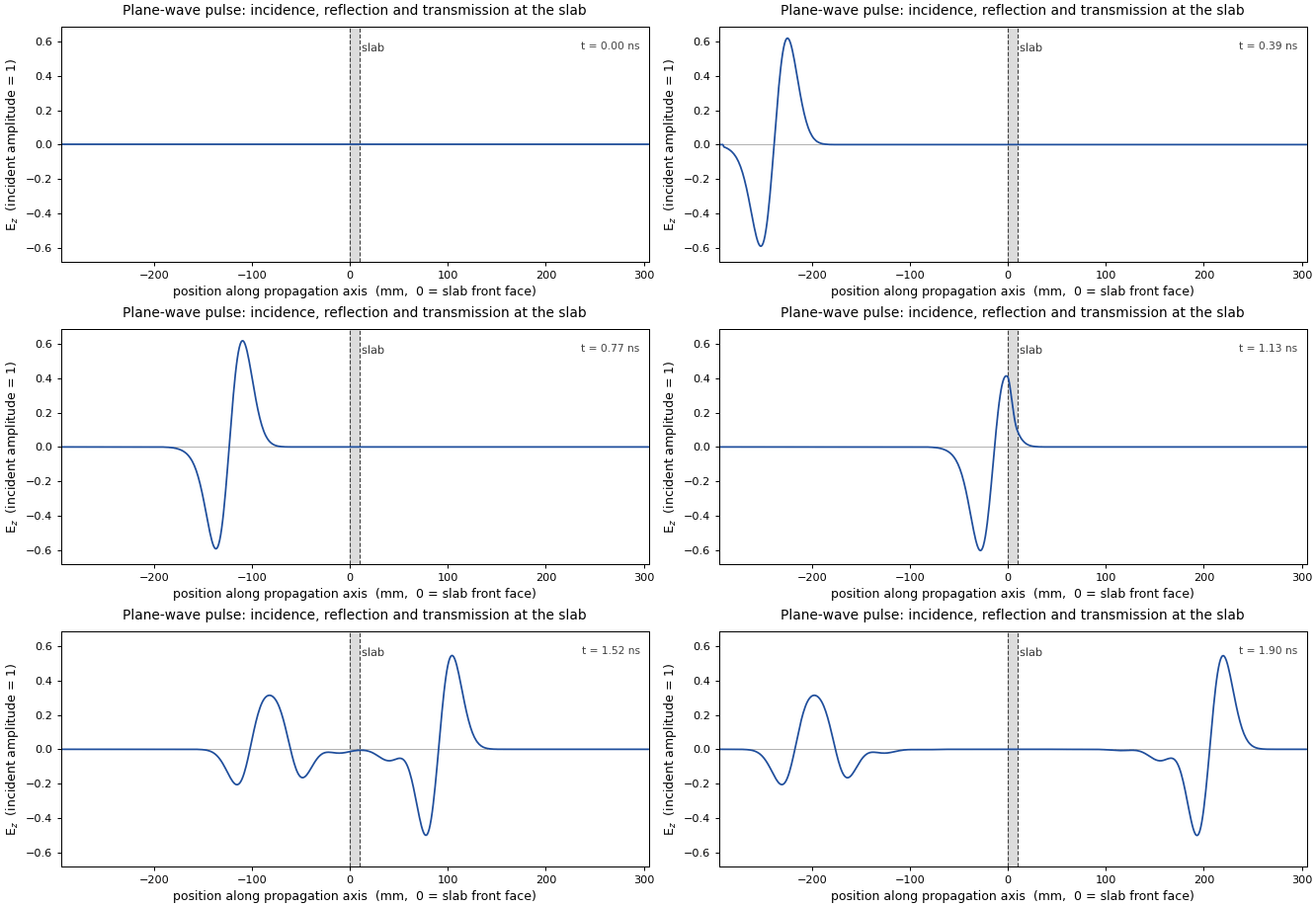
The same run played back in time: the plane-wave pulse travels in at c, hits the slab front face, and splits into a reflected pulse heading back and a transmitted pulse continuing forward (slowed to c/n inside the slab).

Result

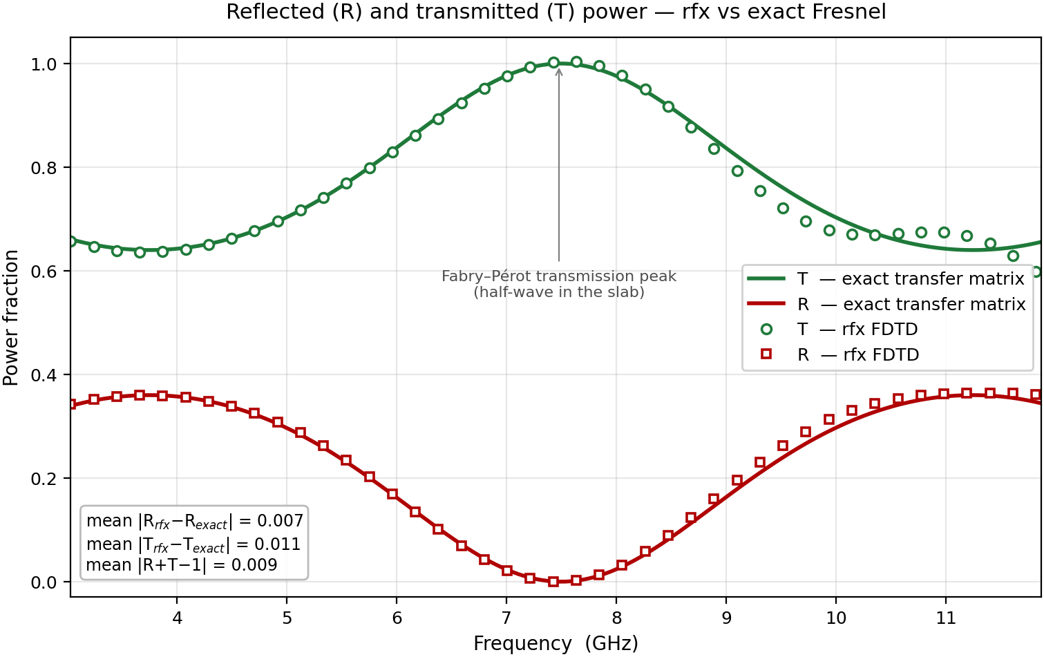
Reflected and transmitted power versus frequency, with the rfx FDTD points laid over the exact transfer-matrix curves. Transmission peaks to 1 (and reflection drops to 0) at the Fabry–Pérot half-wave near 7.5 GHz, exactly where the slab is a half-wavelength thick. Reflection rises toward the band edges where the slab is electrically thinner or thicker than a half-wave.

S-parameter data (Touchstone .s2p) Reflection (S11) and transmission (S21) vs frequency, two-port Touchstone.

Validation & limits

The rfx R/T track the exact Fresnel curves across the full 3–12 GHz band:

Quantity	rfx vs exact	Note
Reflection R	mean |R_rfx − R_exact| ≈ 0.007	absolute power error
Transmission T	mean |T_rfx − T_exact| ≈ 0.011	absolute power error
Energy R + T	mean |R + T − 1| ≈ 0.009	lossless: should be 1

Reference: the exact transfer-matrix (Fresnel) solution. Both errors sit near 1%, well inside the 5% bound this case is held to (mean |R/T error| < 0.05 and |R + T − 1| < 0.05).

The agreement is at the ~1% level and the reflected plus transmitted power adds back to unity, as it must for a lossless slab — a clean independent check that no energy is created or lost at the interfaces.

Where it drifts. The largest deviation is near the top of the band (above ~9 GHz), where the cells are coarsest relative to the wavelength and numerical dispersion shifts the FDTD phase velocity slightly. Refining the mesh from 1 mm toward 0.5 mm pulls the high-frequency points back onto the analytic curve; the half-wave peak near 7.5 GHz is already converged at 1 mm. The model is lossless and normal-incidence only — oblique incidence and material loss would each need their own setup.

Autodiff

The slab is the cleanest place to see what makes rfx different: jax.grad flows straight through the FDTD time stepping. Here the design variable is the slab thickness d and the scalar of interest is the transmission T = |S21|² at one frequency. The thickness enters the permittivity as a soft top-hat — a smoothed slab edge that is a continuous function of d — so a single jax.value_and_grad call returns both T(d) and the sensitivity dT/dd, with the gradient computed by differentiating automatically back through every Yee update of the run.

What makes this the cleanest case is that the slab transfer matrix gives T(d) in closed form, so the derivative has an exact analytic expression:

T(d) = 1 / (1 + F·sin²δ) with F = ((n − 1/n)²)/4 and δ = 2·π·f·n·d/c, giving dT/dd = −T²·F·sin(2δ)·(2·π·f·n/c).

Because the closed form exists, the AD gradient can be checked against the exact derivative directly. Two numbers are reported, because they answer two different questions:

• AD vs central finite differences on the same discretised forward — is the AD machinery itself correct? Here 0.00013 % (rel. error 1.3e-06). The gradient jax.grad returns is the exact derivative of the simulation it ran.
• AD vs the continuum analytic derivative — has the FDTD physics converged to the textbook slab? Here 2.6 % at 0.25 mm cells. The residual is numerical (Yee phase-velocity dispersion plus the one-cell soft edge) and shrinks as the mesh is refined.

Check	AD value	Compared against	rel. error	Sign agrees
AD vs central finite difference	dT/dd = 64.7725	central FD 64.7724 (h = 5e-5)	1.3e-06 (0.00013%)	yes
AD vs closed-form derivative	dT/dd = 64.7725	analytic dT/dd	0.0261 (2.6%)	yes

Both land well inside the 5% agreement asked of them. Read together: the 0.00013% row says the gradient is the exact derivative of the simulation that actually ran; the 2.6% row says how close that simulation is to the textbook slab at 0.25 mm cells — a mesh-refinement question, not a gradient question.

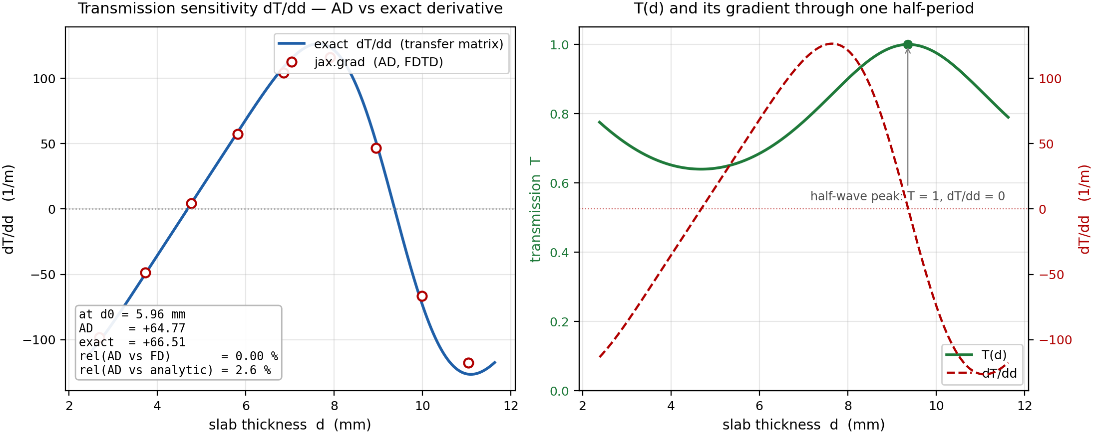
The left panel lays the AD markers on the exact dT/dd curve across a Fabry-Pérot half-period; they sit on the analytic line. The right panel shows T(d) and dT/dd together: the gradient passes through zero exactly at the half-wave transmission peak, where T → 1 and the slab is momentarily insensitive to a small change in thickness. The working point is chosen on a steep mid-slope (δ ≈ 2 rad), not at the peak, where the relative comparison is well posed.

The differentiable knob here is a material/thickness quantity. The number of mesh cells across the slab is a discrete count and is not differentiable; thickness is made smooth on purpose, through the soft top-hat, so that d can be a continuous input to the solver.

Next

Rectangular microstrip patch antenna (2.4 GHz, FR4) A printed resonator: matched return-loss dip, Harminv resonance, and the TM010 field map.

Computed with rfx · 2026-06-24